This manual gives a brief description of Emergent Self-Organizing Maps and visualizations like the U-Matrix. We explain how to use them for data mining using the Databionics ESOM Tools, see also [Ultsch, Moerchen 2005]. The first section briefly introduce ESOM. The following sections give a step by step tour of a typical usage for data mining involving:
The last section covers topics like the command line tools, the Matlab interface, or file formats.We also provide a German manual that is shorter and not as up to date.
For a detailed explanation of SOM, see [Kohonen 1995]. We will give a very brief introduction here.
We assume the training data is a set of points from a high dimensional space, called the data space. A SOM basically consists of a set of prototype vectors in the data space and a topology among these prototypes. The most common topology is a 2-dimensional grid where each prototype (neuron) has four immediate neighbors. The positions on the grid form the map space. Further two distance functions are needed, one for each space. The Euclidean distance is commonly used for the data space and the Cityblock distance for the map space. The process of SOM training adapts the grid of prototype vectors to the given data creating a 2-dimensional projection that preserves the topology of the data space.
A central operation in SOM training is the update of a prototype vector by a vector of the training data. The prototype vector of the neuron is drawn closer to a given vector in the data space. Further, prototypes in the neighborhood of the neuron are also drawn in the same direction but with less emphasis. The emphasis and the size of the neighborhood are reduced during training.
The two most common training algorithms are Online and Batch training. Both search the closest prototype vector for each data point (the bestmatch). In Online training the bestmatch is immediately updates, while in Batch training the bestmatches are first collected for all data points and then the update if performed collectively.
Emergence is the ability of a system to develop high level structures by the cooperation of many elementary processes. In self organizing systems the structures evolve within the system without external influences. Emergence is the appearance of high level phenomena that can not be derived from the elementary processes. Emergent structures offer a more abstract description of a complex system consisting of low level individuums. A popular example of an emergent phenomenon is the so called La Ola wave in a sports stadium. A large number of people perform the simple task of standing up and waving for a short moment. In this way a wave rolling through the crowd is formed. The wave is not visible at the moment of being part of it, only from a distance.
Transferring the principles of self organization into data analysis can be done by letting multivariate data points organize themselves into homogenic groups. A well known tool for this task that incorporates the above mentioned principles is the Self-Organizing Map (SOM). The SOM iteratively adjusts to distance structures in a high dimensional space and gives a low dimensional projection that preserves the topology of the input space as good as possible. Such a map can be used for unsupervised clustering and supervised classification.
The power of self organization that allows the emergence of structure in data is, however, often neglected. We think this is in part due to a misusage of Self-organizing Maps that is widely spread in the scientific literature. The maps used by most authors are usually very small, consisting of somewhere between a few and some tens of neurons.
Also the concept of border less maps (e.g. toroid maps [Ultsch 2003b]) to avoid border effects is rarely used. Using small SOM, is almost identical to a k-Means clustering with k equal to the number of nodes in the map. The topology preservation of the SOM projection is of little use when using small maps. Emergent phenomena involve by definition a large number of individuums, where large means at least a few thousand. This is why we use large SOMs and called them Emergent Self-Organizing Maps (ESOM) [Ultsch 1999] to emphasize the distinction. It has been demonstrated, that using ESOM is a significantly different process from using k-Means [Ultsch 1995].
When using supervised neural nets, e.g. multi layer perceptrons trained with Backpropagation, a common concern is the model size. Too small neural nets have low accuracy, while too large nets are prone to over-fitting. Note, that this is not the case with ESOM. Using larger maps does not really increase the degrees of freedom in the same sense, because the neurons are restricted by the topology preservation of the map. Using large maps should rather be viewed as increasing the resolution of the projection from the data space onto the map.
A very important step prior to ESOM training is preprocessing of the data. For each feature the empirical probability distribution should be analyzed e.g. with histograms or kernel density estimates. If the distribution is skewed we recommend using non linear transformations (e.g. log) to make is more symmetric. Outliers can be detected e.g. using box plots or statistical tests. These extreme values can be interesting in some applications, but they should be removed prior to SOM training because they will severely distort the grid and can hide the more interesting clustering structure. The correlation among features is another important aspect. If several features are highly correlated, this may introduce unwanted emphasis of this aspect of the data. The Pearson correlation coefficient and scatter plots can be used to detect correlation. Some features can then be discarded. Finally, for meaningful distance calculations, the means and variances of the features should be made comparable. This is commonly done using the z-transformation to have zero mean and unit variance for all inputs and thus provide an equal weighting in distances. For more information see e.g. [Hand et al. 2001].
The complete process of preprocessing is beyond the scope of the Databionic ESOM Tools. But we do provide the possibility to normalize the values by pushing the one of the buttons in the toolbar of the data tab. Z-transform applies column-wise normalization to zero mean and unit variance. Robust ZT does the same but uses robust estimates of mean and variance. Finally, to [0,1] rescales each column to range from zero to one.
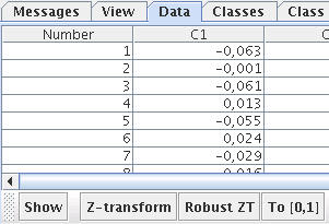
After starting up the ESOM Analyzer (with the start menu or the command esomana) you need to load the data in the application with the File->Load *.lrn menu item. The data needs to be in the *.lrn format, basically tab separated values in a text file. The menu item Tools->Training opens up the training dialog. The options are explained here.

Press Start to train the ESOM. The output of the training program will be shown, e.g. the epoch and the current quantization error. You can cancel the process by pressing the Stop button. When the training is finished press the Close button to return to the main window.
This section describes how ESOM can be visualized and analyzed using the tools in the View tab at the bottom.

The result of ESOM training is a low dimensional grid of high dimensional prototype vectors. The positions of the bestmatches for the data points alone does often not offer an intuitive visualization of the structures present in the high dimensional space. Additional methods are needed to visualize the structures based on distances and densities in the data space. You can select a visualization from the Background drop down list. The check box can be used to turn off the background.
The U-Matrix [Ultsch 1992] is the canonical display of ESOM. The local distance structure is displayed at each neuron as a height value creating a 3D landscape of the high dimensional data space. The height is calculated as the sum of the distances to all immediate neighbors normalized by the largest occurring height. This value will be large in areas where no or few data points reside, creating mountain ranges for cluster boundaries. The sum will be small in areas of high densities, thus clusters are depicted as valleys.
See the reference for a description of the other backgrounds. You can further change the appearance of the background with the following controls.
| Gradient | Select a color gradient to be linearly mapped on the height values. The smallest height will be mapped to the leftmost value, the largest to the rightmost. The number of color steps can be down sampled with the Colors option below. |
| Contours | A black line is drawn between each color, creating contour lines of equal height. Best used with a small value of the Colors option. |
| Colorize | Semi-transparent color based on the Opinion background. Should be used with gray gradient. Slow. |
| Tiled display | For border less grids the visualizations should be viewed in tiled mode, displaying four copies of the grid. This way clusters stretching over the edge of the grid image can be seen connected. Unfortunately this also means that every data point and cluster is visible in 4 different places. This can be compensated by extracting a map from the tiled view removing the redundancies. |
| Zoom | The zoom factor controls size of the visualization. Each neuron will be displayed with zoom x zoom pixels. |
| Colors | The number of color steps to use from the gradient. |
| Clip | If there are some extreme height values, e.g. because of high dimensional outliers, the remaining structure of the ESOM will be hidden, because the heights are normalized to the interval [0,1]. Clipping can be used to map a percentage of the largest heights to 1 and offering more resolution to the smaller heights. |
The Component tab at the bottom can be used to restrict the calculation of background visualization to to a subset of the features. Deselect features by un-checking them and press update.

The Legend tab at the bottom displays a legend for the color steps in form of a histogram. The height of each bins corresponds to the number of neurons with this color. A click on the legend toggles the histograms display an a plain legend. The latter can be useful if some colors are underrepresented and the bars almost flat. The Legend can be saves as an image using the menu item File->Images->Save legend.

The foreground display draws the bestmatches on top of the background and can be controlled with the remaining options in the View tab. Each neuron that is a bestmatch for at least one data point is marked with a point on the map. The default color of the points can be set in the Options tab.
| Bestmatch size | The size of the squares/circles drawn for each data point. |
| Draw Bestmnatches | Whether to draw squares/circles for data points. |
| Opinion coloring | Color squares/circles for data points with colors from Opinion background. |
| Show names | Display names for data points loaded from *.names file. |
| Round Bestmnatches | Draw circles instead of squares for data points. |
If you saved intermediate results during the ESOM training using the save *.wts and *.bm every n-th epoch, you can create an animation of the training process. Select the Slide Show tab and press the Generate button. A series of pictures based on the current display settings will be created. You can view the slide show with the Open button. The playback controls at the bottom enable forward, backward, and stepwise animation. The slider changes the speed.
The Island mask tab can be used to remove the redundancy present in a tiled display of a border less ESOM. A tiled display shows the original ESOM four times to display clusters stretching over the edge of the map. The mask will cover duplicate neurons and creating a so-called map display where each neuron is visible at most once. The rightmost toolbar button is automatically selected. Use the mouse similar to the data selection mode to select an area of the ESOM. The remaining areas are filled with water. There are two modes of cutting:
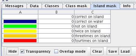
The transparency checkbox turns tranparency on and off for water and overlap mask.
The show/hide button toggles visibility of water and overlap mask.
The island mask can be saved and loaded to an *.imx file.
The data tab displays the loaded data file (*.lrn) and optionally the loaded names (*.names) and classification (*.cls). The data entries, column names, and dataset names can be edited in place. The changes can be saves to *.lrn and *.names files with the menu items in the file menu.

The mouse can be used with the Ctrl and Shift keys to select table entries in the usual manner. The corresponding bestmatches on the map will be highlighted. You can also select bestmatches on the map with the mouse using the selection tool (the rightmost toolbar button automatically activated along with the data tab). The mouse tool can be used to draw a line around a set of bestmatches. Keeping the left mouse button pressed creates a freehand line, several clicks with the left mouse button create a polygon. Pressing the right mouse button finishes the line by connecting the end with the beginning. Using the mouse with the Ctrl pressed can be used to select additional points without discarding the previous selection. Selecting points with the Shift key pressed will remove them from the current selection. The popup menu offers more options for selection. The hide/show button can be used to toggle the display of the selection without discarding it.
The data table popup menu can be used to remove the selected data points. This is useful if you identify high dimensional outliers. On a U-Matrix these will be visible by a large mountain range surrounding a single or a few bestmatches. After outlier removal you should retrain the ESOM with the remaining data. The File->Selection menu items can be used to store the selection in a separate *.lrn file of create a classification with the selection in class 1 and the rest in class 0.
The clustering of the ESOM can be performed at two different levels. First, the bestmatches and thus the corresponding data points can be manually grouped into several clusters. Secondly, the neurons can be clustered. This way regions on the map representing a cluster can be identified and used for classification of new data. In neither case all elements need to be labeled.
The dataset used for training an ESOM can be clustered manually by looking at the ESOM visualizations. The U-Matrix is a visualization of the local distance structure in the data space. It's values are large in areas where no or few data points reside, creating mountain ranges for cluster boundaries. Small values are observed in areas where the data space distances of neurons are small, thus clusters are depicted as valleys. Similarly the P-Matrix can be used for density based clustering, by selecting areas with large values as clusters. The manual clustering of an ESOM is comparable to manually selecting cluster from a dendrogram representation for hierarchical clustering algorithms.
The Classes tab and the corresponding second mouse tool in the toolbar can be used to cluster the bestmatches and thus the datasets manually. Datasets can be selected on the map analogous to the data selection mode explained above. Pressing the right mouse button creates a new entry in the class table. the corresponding bestmatches will be displayed in a new color. The checkbox in the table can be used to highlight a class, the color and name of the class can be edited in the table. The popup menu can be used to remove classes or start over. The Hide/Show button can be used to toggle the coloring of the bestmatches. Names for the classes can be entered directly in the table and the first letter of the class name can be displayed on the map by selection the checkbox Draw letters. The map space of each class can be calculated. The map space corresponds to a 1-nearest neighbor classification of all neurons according to the current classification of the bestmatches. This indicates how much rooma class is occupying on a map.
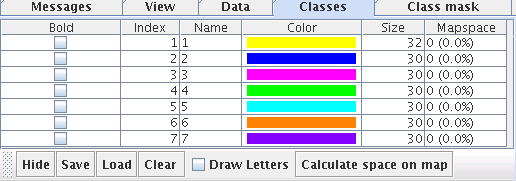
The clustering result can be saved in a *.cls file. The file will have the same number of rows as the *.lrn file using the unique identifiers for each dataset. Datasets with no class are assigned to the default class with index 0.
Clustering the bestmatches of an ESOM usually does only lead to a clustering of the original training data. The projection of new data points on the map will however surely hit map neurons without a bestmatch and thus without a label. Labeling all (or most) neurons instead of only the bestmatches solves this problem. One essentially creates a sub-symbolic classificator similar to a k-nearest neighbor (KNN) classifier with $k=1$ that can be applied to new data automatically. The main difference to KNN is, that the user can use the visualization of the ESOM to create the labeling whereas KNN does not offer this convenience. Further KNN classification always classifies a point, no matter how near (or rather far) the neighbors are. In contrast, ESOM classification offers a don't know class by leaving neurons unlabeled, e.g. for sparsely populated regions separating clusters. When using distance based visualizations, map regions indicating large distances in the data space should not be labeled. These regions correspond to the empty space between two more populated regions. If a new data point lies in this region his bestmatch will be an interpolating neuron without a label. Similarly, sparse regions can be spared when using density-based visualizations.
The Class mask tab and the corresponding third mouse tool in the toolbar can be used to cluster the neurons. The handling is analogous to the bestmatch/data clustering, only the clusters are displayed as semi-transparent colored areas on top of the background.

The clustering result can be saved in a *.cls file. The file will have the same number of rows as the *.wts file using unique identifiers for each neuron. Neurons with no class are assigned to the default class with index 0.
The projection of data onto an ESOM means finding the bestmatches for each data point. This task can be performed by loading an ESOM (*.wts) or using newly trained ESOM, loading a new data file (*.lrn) and selecting the menu item Tools->Project. The bestmatches will be calculated, displayed on the map and can be saved using the menu item File->Save (*.bm).
The class mask created by clustering the neurons of an ESOM can be used for classification. Each bestmatch and thus the accompanying dataset(s) is assigned to the class of the region it resides in. Bestmatches not covered by a class mask are placed in the default class 0. Classification can be performed by loading bestmatches (*.bm) or using the bestmatches of a newly trained ESOM and loading or creating a class mask (*.cls) with the menu item File->Class mask->Load. Selecting the menu item Tools->Classify will label all bestmatches and display the result as colors on the map and in the Classes tab. The classification can be saved using the menu item File->Save (*.cls).
| input file | The input *.lrn file, set automatically. | ||
| output files | The generated output files, set automatically. The *.wts file contains the weights of the trained ESOM, the *.bm lists the positions of the bestmatches, and the *.umx file stores the heights of a U-Matrix. | ||
| training algorithm |
| ||
| k for k-Batch as percentage of data set | Percentage of all data vectors that is processed between map updates. | ||
| threshold for Hybrid-Batch as percentage of map size | The minimum percentage of data points that is required to be placed on a different bestmatches. Other wise one epoch of Online learning is performed. | ||
| number of rows in map | The vertical size of the ESOM grid. | The product of rows and columns, i.e. the number of neurons should be at least 1K neurons. The ratio of rows and columns should be significantly different from unity. | |
| number of columns in map | The vertical size of the ESOM grid. | ||
| number of training epochs | The number of iterations over the training data. | ||
| search method for bestmatches |
| ||
| radius for local bm search methods | If the 'quick learning' bestmatch search strategies are active this is the constant that is added to the current radius of the learning neighborhood. If the 'local search with constant radius' is active this is the fixed search radius. | ||
| weight initialization method | The prototypes of the ESOM can be initialized randomly by
| ||
| data space distance function | The distance function to use for bestmatch search. The Lp distances are available for p = 1/4,1/3,1/2,1(=Manhattan),2(=Euclid),3,4,inf(=Maximum). Further you can select the Cosine and Correlation distances. All distances are available as a version ignoring missing values (NaN). If you data does not have missing values, the using the plain version will be faster. | ||
| start value for radius | The initial value for the radius of the neighborhood around each neuron used for updating. Should be on the order of half the smaller length of the grid. | ||
| final value for radius | The final value for the radius of the neighborhood around each neuron used for updating. Use 1 for a high level of detail of the final map and larger values for more emphasis of coarser structures. | ||
| cooling strategy for radius | The radius of the neighborhood is cooled down during training. You can choose the function for the radius w.r.t. to the training episode.
| ||
| start value for learning rate | The initial value for the learning rate used for updating. | ||
| final value for learning rate | The final value for the learning rate. | ||
| cooling strategy for learning rate | Same as for the radius, no cooling is possible though. | ||
| map grid (and grid distance) | The topology of the ESOM grid the the distance function in the map space. There are two topologies: with borders or toroid/border-less grids. The toroid topology avoids border effects by connections the top of the map to the bottom and the left to the right (see images). The distance functions on the grid correspond to the shape of the neighborhood: Manhattan (diamond), Euclidean (circle), Maximum (square). |
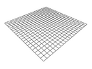
Planar topology with borders. |
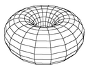
Toroid topology without borders. |
| Note: we only use quad-grids where each neuron hat four immediate neighbors. The popular hex-grid with six immediate neighbors is implemented in the training part of the Databionics ESOM Tools but not in the visualizations part. Recent studies indicate the the shape of the map is more important for topology preservation than the number of immediate neighbors [Ultsch 2005]. |
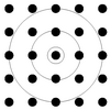
Quad-grid neuron placement. |
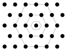
Hex-grid neuron placement. | |
| neighborhood kernel function | The weighting kernel of the neighborhood used for updating.
|

Cooling functions plotted from center to edge of neighborhood. | |
| permute data patterns | The data points are shuffled before each new training episode. Recommended. | ||
| save *.wts and *.bm every n-th epoch | This can be used to create an animation of ESOM training with the slide show function. | ||
| save *.umx for each *.wts | For convenience a U-Matrix can be saved for each *.wts file. | ||
| U-Matrix | The U-Matrix [Ultsch 1992] is the canonical display of ESOM. The local distance structure is displayed at each neuron as a height value creating a 3D landscape of the high dimensional data space. The height is calculated as the sum of the distances to all immediate neighbors normalized by the largest occurring height. This value will be large in areas where no or few data points reside, creating mountain ranges for cluster boundaries. The sum will be small in areas of high densities, thus clusters are depicted as valleys. |
| TwoMatch | The TwoMatch display is a variation of the U-Matrix using the distances to the two closest bestmatched. |
| P-Matrix | While distance-based methods usually work well for clearly separated clusters, problems can occur with slowly changing densities and overlapping clusters. Density based methods more directly measure the density in the data space sampled at the prototype vectors. The P-Matrix [Ultsch 2003b] displays the local density measures with the Pareto Density Estimation (PDE) [Ultsch 2003a], an information optimal kernel density estimation. |
| Component | The component visualization depicts the distributions of single features values on the map. One picture for each feature is drawn, you can restrict the display to fewer components using the Component tab at the bottom. Deselect features by un-checking them and press update. |
| Gap | The Gap visualization inspired by the method proposed in [Kaski 2000]. The aim is to search for low-density regions with a change in the gradient of the sample density, called gaps. The distance to a local centroid is used as a indicator for gaps. The local centroid is the mean of the immediate neighbors. |
| Opinion | The Opinion visualization does not create height values that are displayed with a color gradient. A color value for each neuron is directly calculated from a high dimensional data vector by using every third value to determine the red values. The blue and green components are calculated similarly with an offset of one and two respectively. |
| Random | The Random background is a dummy method that produces random height values for comparison. |
| SDH | The Smoothed Data Histograms (SDH) [Pampalk et al. 2002] use a rank based measure to approximately display the data density. The grid is interpreted as a high dimensional histogram where the Voronoi regions of the prototype vector act as bins. A data points adds (decreasing) weights only to it's k closest bins. This way large values are observed where the data density is high because the bins get many weights. Low values are obtained in regions with low density because a prototype well be among the k closest to few or no data points. |
The *.lrn file contains the input data as tab separated values. Features in columns, datasets in rows. The first column should be a unique integer key. The optional header contains descriptions of the columns. Missing values can be given an '?' or 'NaN'.
# comment # % n % m % s1 s2 .. sm % var_name1 var_name2 .. var_namem x11 x12 .. x1m x21 x22 .. x2m . . . . . . . . xn1 xn2 .. xnm |
| n | Number of datasets. |
| m | Number of columns (including index). |
| si | Type of column: 9 for unique key, 1 for data, 0 to ignore column. |
| var_namei | Name for the i-th feature. |
| xij | Elements of the data matrix. Decimal numbers denoted by '.', not by ','. |
Classification files contain a class assignment for datasets or neurons. The optional header contains names and colors for the classes.
# comment # % n %c_1 s_1 r_1 g_1 b_1 %c_2 s_2 r_2 g_2 b_2 %... %c_m s_m r_m g_m b_m id_1 cl_1 id_2 cl_2 .. .. .. .. .. .. id_n cl_n |
| n | Number of datasets. |
| m | Number of classes. |
| c_j | Class number. |
| s_j | Class name. |
| r_j | Red component of class color. |
| g_j | Green component of class color. |
| b_j | Blue component of class color. |
| id_i | Index of i-th dataset. |
| cl_i | Classification of i-th dataset. |
Names files contain short and long names for each dataset.
% n key_1 short_1 long_1 key_2 short_2 long_2 .. .. .. .. .. .. key_n short_n long_n |
| n | Number of lines. |
| key_i | Integer key |
| short_i | Short name, usually a few letters. |
| long_i | Longer description. |
The *.wts file contains the weight vectors for all neurons of an ESOM. Each entry is one vector of the same length as the vectors in the input data.
# comment # # % k l % m w001 w002 .. w00m w011 w012 .. w01m w021 w022 .. w02m . . .. . w0(l-1)1 w0(l-1)2 .. w0(l-1)m w101 w102 .. w10m w111 w112 .. w11m . . .. . w1(l-1)1 w1(l-1)2 .. w1(l-1)m . . .. . . . .. . w(k-1)(l-1)1 w(k-1)(l-1)2 .. w(k-1)(l-1)m |
| k | Number of rows of the ESOM |
| l | Number of columns of the ESOM |
| m | Number of features in the dataset |
| wijh | h-th component of the weight that can be found in row i and column j on the map. The position (0,0) is in the top left corner of the map. |
The weights are positioned as follows:
(0,0) (0,1) (0,2) ... (0,l-1) (1,0) (1,1) (1,2) ... (1,l-1) ... |
In the sequence of their appearance in the *.wts-file the vectors are transformed into the map as follows:
0 1 2 ... l-1 l l+1 l+2 ... 2l-1 ... |
The *.bm file contains the index of a data point and the coordinates of it's best match. The best match is the neuron, on which the data-point is projected by the training algorithm.
% k l % n index1 k1 l1 index2 k2 l2 . . . . . . indexn kn ln |
| k | Number of rows of the feature map. |
| l | Number of columns of the feature map. |
| indexi | Index of best match i. Corresponds to the index of the i-th data-point in the *.lrn file. |
| ki | Row of the i-th best match. |
| li | Column of the i-th best match. |
The *.umx file contains a height value for each neuron of an ESOM, e.g. the elements of the U-Matrix.
% k l h11 h21 h31 .. hk1 h12 h22 h32 .. hk2 . . . .. . . . . .. . h1l h2l h3l .. hkl |
| k | Number of rows of the ESOM. |
| l | Number of columns of the ESOM. |
| hij | Height of the neuron at position i in x-direction and j in y-direction. |
Many of the functionality of the Databionic ESOM Tools are also available from the command line. The help for the command line parameters can be displayed by running the command with the -h switch.
| esomana | Starts the ESOM Analyzer GUI. You can specify filenames to be automatically loaded. |
| esomcls | Loads a class mask (*.cmx) and bestmatches (*.bm) and saves the result of the classification of the bestmatches (*.bm). |
| esomprj | Loads a trained ESOM (*.wts) and a dataset (*.lrn) and saves the bestmatches for the data on the grid (*.bm). |
| esommat | Loads a trained ESOM (*.wts) and optionally a dataset (*.lrn). Saves a matrix of height values (*.umx). |
| esomrnd | Loads a trained ESOM (*.wts) and optionally a dataset (*.lrn) and a classification (*.cls). Saves an image (*.png). |
| esomtrn | Loads a dataset (*.lrn) and trains an ESOM. The weights (*.wts) and final bestmatches (*.bm) are saved. |
The Databionic ESOM Tools include an interface for calling from within Matlab. Further, functions for loading and saving the ESOM file formats are included. To install it you need to include the matlab folder and all subfolders in your Matlab path.
| load* | Load a file formats: *.bm, *.cls, *.lrn, *.names, *.rgb, *.umx, *.wts |
| save* | Save a file formats: *.bm, *.cls, *.lrn, *.names, *.rgb, *.umx, *.wts |
| esomtrain | Loads a dataset (*.lrn) and trains an ESOM. The weights (*.wts) and final bestmatches (*.bm) are saved. |
| esompicture | Loads a trained ESOM (*.wts) and optionally a dataset (*.lrn) and a classification (*.cls). Saves an image (*.png) and optionally the matrix of height values (*.umx). The image is displayed in Matlab. |
| esomprojection.m | Loads a trained ESOM (*.wts) and a dataset (*.lrn) and saves the bestmatches for the data on the grid (*.bm). Given a neuron classification, new data can be classified. |
| esom_map_tool.m | Starts the ESOM GUI. You can specify filenames to be automatically loaded. |
| [Noecker et al. 2006] Noecker, M., Moerchen, F., Ultsch, A.: Fast and reliable ESOM ESOM learning, In Proc. ESANN 2006, (2006) |
| [Ultsch 2005b] Ultsch, A., Moerchen, F.: ESOM-Maps: tools for clustering, visualization, and classification with Emergent SOM, Technical Report Dept. of Mathematics and Computer Science, University of Marburg, Germany, No. 46, (2005) |
| [Ultsch 2005] Ultsch, A., Herrmann, L.: Architecture of emergent self-organizing maps to reduce projection errors, In Proc. ESANN 2005, pp. 1-6, (2005) |
| [Ultsch 2004] Ultsch, A.: Density Estimation and Visualization for Data containing Clusters of unknown Structure., In Proc. GfKl 2004 Dortmund, pp. 232-239, (2004) |
| [Ultsch 2003b] Ultsch, A.: Maps for the Visualization of high-dimensional Data Spaces, In Proc. WSOM'03, Kyushu, Japan, pp. 225-230, (2003) |
| [Cuadros-Vargas et al. 2003] Cuadros-Vargas, E., Romero, R.A.F., Obermayer, K.: Speeding up algorithms of SOM family for large and high dimensional databases, In Proc. WSOM'03, Kyushu, Japan, pp. 167-172, (2003) |
| [Kinouchi et al. 2003] Kinouchi, M., Yoshihiro. K.: Much faster Learning algorithm for Batch-Learning SOM and its application to Bioinformatics, In Proc. WSOM'03, Kyushu, Japan, pp. 107-111, (2003) |
| [Ultsch 2003a] Ultsch, A.: Pareto Density Estimation: Probablity Density Estimation for Knowledge Discovery, In Innovations in Classification, Data Science, and Information Systems, Springer, pp. 91-102, (2003) |
| [Pampalk et al. 2002] Pampalk, E., Rauber, A., Merkl. D.: Using Smoothed Data Histograms for Cluster Visualization in Self-Organizing Maps, In Proceedings ICANN'02, (2002) |
| [Hand et al. 2001] Hand, D., Mannila, H., Smyth, P. E.: Principles of Data Mining, MIT Press (2001) |
| [Kaski et al. 2000] Kaski, S., Nikkil, J., Kohonen, T.: Methods for exploratory cluster analysis, In Proceedings of SSGRR 2000, (2000) |
| [Ultsch 1999] Ultsch, A.: Data Mining and Knowledge Discovery with Emergent Self-Organizing Feature Maps for Multivariate Time Series, In Kohonen Maps, (1999) , pp. 33-46 |
| [Ultsch 1995] Ultsch, A.: Self Organizing Neural Networks perform different from statistical k-means clustering, In proceedings GfKl, Basel, (1995) |
| [Kohonen 1995] Kohonen, T.: Self-Organizing Maps, Springer (1995) |
| [Ultsch 1992] Ultsch, A.: Self-Organizing Neural Networks for Visualization and Classification, In Proc. Conf. Soc. for Information and Classification, Dortmund, April, (1992) |